
The best known and used methods of Chemometrics and Machine Learning are presented here below.
-
Methods of exploratory analysis
Principal Component Analysis
Principal Component Analysis (PCA) is the major workhorse of the chemometrics tools. PCA method can be used for the following goals:
- Visualisation of X in the multivariate space
- Cluster detection
- Outlier detection
- Effect of variability factors
- Data compression, when reducing X dimensionality
- Noise removal
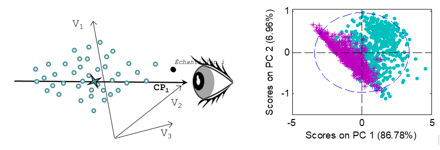
PCA can be seen as a better way to visualize samples represented by numerous variables, by projecting their original coordinates into a new set of axes, called Principal Components (PC). These axes are built so as to maximize the variance of X, thus extracting the information. The first k components represent the summarized information of X, the last components represent the noise.
Thus, PCA can be seen as a change of axes, designed to better visualize the sample variability, but maintaining the distances and scales between samples. For more convenience, the samples are usually visualized on a 2D ou 3D plane, corresponding to the projection of the samples on this set of 2 or 3 axes
PCA can be the basics for other multivariate methods, such as unsupervised classification or Multivariate Statistical Process Control (MSPC).
Multi-blocks Analysis
Multi-block data sets include data sets where
- the same samples are characterized with different blocks of variables, the nature and the number of variables of these different blocks can vary
- or several blocks of samples are characterized with the same variables, the number of samples in each block can be different.
The goal of Multi-block analysis is to identify common and specific information within the different blocks of data.

Independent Component Analysis
ICA aims at identifying the products and phenomena present in a mixture, or during a process. The main components of a PCA, which most often describe a mixture of these pure sources, do not always provide an adequate response.
The basic assumption of the ICA is to consider each row of matrix X as a linear combination of “source” signals, S, with weighting coefficients, or “proportions”, A, proportional to the contribution of the source signals in the corresponding mixtures.
Unlike PCA, the results depend on the number of components you want to extract. Thus, for an ICA with 3 components for example, the first component will be different from that of an ICA performed on 4 components. Some tools exist to make easier the choice of the number of components, such as for example “ICA by block”, which makes it possible to check the robustness of the model by looking at the correlations between the components of ICA models made on data split in blocks.
-
Unsupervised Classification (clustering) :
For classification purposes, there are two ensembles of methods.
The first one are the “unsupervised classification” methods (or clustering) which aim at regrouping similar samples without the use of prior knowledge. The second one are the “supervised classification” methods (or discrimination), where class memberships are used to build a model.
The clustering techniques are also called “unsupervised classification” techniques in the chemometrics field or “data-mining” techniques in the machine learning field. They are exploratory tools which aim at finding “natural” clustering trends out of the inner data structure (X) without any other prior knowledge on the class assignment of the samples. Thus, all these methods measure the similarities between samples only according to their X values.
Hierarchical Clustering Analysis (HCA)
Hierarchical Clustering Analysis is a method which assembles or dissociates successively sets of samples. In Agglomerative Hierarchical Classification, n classes are considered at the beginning, i.e. one class per sample, and are regrouped successively until it constitutes a unique class.
The result is given in a form of a tree, called dendrogram, where the length of the branches represents the distance between groups. The choice of the final groups is decided by cutting at a threshold, defined by the user; thus the number of clusters is not a parameter to be set beforehand.
However, two other criteria must be defined: the distance between samples (generally the Euclidean distance) and the grouping criterion. Different trees are indicated in the figure depending on the grouping criterion chosen. The impact on the classification is quite visible in this figure.

K-Means
Non-hierarchical clustering methods aim at building one final partition of the data. Contrarily to the hierarchical approach, the user must set a fixed number of groups out of his prior knowledge, which can be a strong limitation to these techniques.
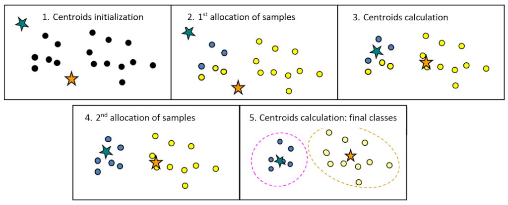
The widely used K-means method is an iterative procedure used to find the best partition of k classes.
The initial partition of k groups is generally generated at random. K-means results are highly dependent on the initial partition and on the choice of the number of classes k.
Then, for each iteration, the barycentre of each class (i.e. the mean vector of the class) is recalculated and the samples are assigned to the nearest centre.
This procedure is carried out until the end criterion is reached (for instance: no assignment changes or maximum number of iterations reached).
-
Regression methods MLR, PCR, PLS :
MLR – Multiple Linear Regression
Multiple Linear Regression (MLR) is the simplest multivariate modeling method. It is the extent of the simple linear regression to the multivariate case.
This method has the advantage of being straightforward. However, if the explanatory variables are correlated (colinearity), the pseudo-inverse matrix calculation leads to unstable models. Another important limitation is that MLR cannot be calibrated if the number of samples is smaller than the number of variables. These two limitations are very often encountered in spectroscopy or imaging where the variables are numerous and strongly collinear. Thus, other modelling methods must be adopted for this kind of data.

PCR – Principal Component Regression
In order to overcome the problems inherent in the MLR method, i.e. the management of colinear data and / or if the number of variables is greater than the number of samples, two steps can be processed:
- The first step consists in applying a PCA on X and extracting from it k informative components (not noisy).
- The components thus extracted can then be used in an MLR instead of X
This method is called Principal Component Regression (PCR). Its disadvantage is that the PCA components are not calculated according to their link with the parameter Y but only according to the maximum variance of X. Y is not always linked to the most important variations in X. Thus, the models are not always very efficient.
PLS – Partial Least Square Regression
Partial Least Squares regression is the most used method in Chemometrics.
Rather than calculating components using only X-variance as PCA does, the PLS algorithm takes into account the covariance between the variables X and y, i.e. the variances of X and y and the correlation between them.
Components, referred here as latent variables (LV), are then built in order to model y. PLS is thus usually more performing than PCR.
The fewer the number of latent variables, the more robust the model is, i.e. stable with respect to external disturbances, but the more it risks being underfitted. It is therefore necessary to choose the number of latent variables carefully in order to create a performing and robust model.
-
Supervised discrimination
SIMCA – Soft Independent Modeling of Class Analogy
Soft Independent Modeling of Class Analogy (SIMCA) is based on PCA (Principal Component Analysis) and is thus suitable for high dimensional data.
Each class k is modeled by a specific PCA. This PCA allows to model the intra-class variance. Then, for each model a confidence interval is built to define the membership limit of the class. This limit can be based on the Euclidean distance of the X-residuals (called Q), on the leverage (or equivalent the Hotelling’s T² or the Mahalanobis distance) or, more often, on the combination of both criteria.
An unknown sample is then classified in class k if it falls within the class limits. A sample can be assigned to several classes if they overlap or are very close to each other, or to none of the classes. In this case, it is possible to consider a “rejection class.
The advantage of SIMCA over other methods of discrimination is that it is very easy to add new classes. Indeed, PCA models are produced by class independently of the other classes.
This method works very well for authenticating products with very different X values. On the other hand, when the signals are very close, methods based on the inter-class differences will be preferable.
PLS-DA – PLS Discriminant Analysis
PLS-DA is a method derived from PLS that allows qualitative analysis or discriminant analysis.
As with PLS, the construction of the PLS-DA model is based on the X and y covariance. But unlike PLS, the y of PLS-DA are not continuous values. Each column matrix of y corresponds to a class and contains either 1 if the sample belongs to the class, or 0 otherwise (a complete disjunctive coding).
Unlike SIMCA, PLS-DA focuses on separating the classes . On the other hand, if the classes are very heterogeneous, this can complicate the modeling because all the samples of the class are assigned to the same quantitative value (1), whereas they are truly different somehow.
The predictions are continuous values because the model still remains a PLS. A new sample will be assigned to the class if its prediction is close to 1 for the associated column. A threshold is usually defined to decide whether or not the sample is assigned to the class, as shown in the figure.

-
Machine Learning methods
SVM – Support Vector Machines
SVM (Support Vector Machines) method is mostly used for non-linear or complex problems. It is based on the search for boundaries to separate two classes. Thus, only a part of the calibration samples is actually used: they are the support vectors that delimit the boundaries.
The data are transformed into a new space, called the kernel, which makes it possible to model non-linearity. In calibration, the dimension of this matrix is nxn (n being the number of samples in calibration). The most common kernel is the Gaussian kernel which requires a Gaussian width optimization parameter: sigma that allows to adjust the degree of non-linearity. The SVM method also requires the optimization of a regularization parameter which makes it possible to avoid overfitting (C or cost). The adjustment of these two parameters is crucial to obtain a model that is both efficient and robust.
Although originally created for classification, SVM methods have been extended to regression, in particular two methods: SVM-R and LS-SVM.

ANN – Artificial Neural Networks
Artificial neural networks (ANN), or shallow networks (to differentiate them from deep learning methods), are modeling tools imitating the biological principle of neurons. The most used Artificial Neural Network is the Multi-Layer Perceptron (MLP). It is organized in layers of interconnected neurons (fully connected), with, at least 3 layers:
- 1 input layer corresponding to the variables X (1 neuron per column)
- 1 or more hidden layer (s) of k neurons that correspond to the weights which will have to be trained to build the model
- 1 output layer corresponding to the Y (1 neuron per column).

They can be quantitative values to be predicted or classes according to the type of network developed. ANN are non-linear stochastic methods, i.e. each modeling process will lead to a different result. It is generally recommended to carry out several iterations.
Non-linearities are managed by the use of activation functions at the output of each neuron from the hidden layer(s). Different kinds of activation functions exist (tangent, sigmoid, etc.).
Weights are adjusted by running through each sample of the calibration set several times. A stopping criterion is then necessary to avoid over-fitting. These methods are therefore to be used with caution, but modeling tips make it possible to obtain robust models.
LWR – Locally Weighted Regression
LWR (Locally Weighted Regression) can be useful in case of non-linearity, or for heterogenous or clustered data.
The principle of this method is to compute a linear regression model for each sample, using only a defined number of its closest neighbors selected from the calibration database rather than the entire population:
- For a sample to be predicted, the neighbors are selected based on their proximity in a PCA calculated globally on all the calibration samples (X values).
- The proximity of the response to predict (Y values) could also be taken into account to influence the selection of the closest samples. The response of the sample to be predicted can be estimated by a global model and compared to the known responses of the calibration samples.
- A local PLS (or PCR) model is then calibrated for the sample to be predicted, using only the selected neighbors.

This results in a “piecewise linear” model based on the range of X and Y, that allows to handle non-linear relationships between X and Y.
CART – Classification And Regression Trees
Classification and Regression Trees (CART) successively split the data into two groups, forming a binary tree.
At each node of the tree, a variable is selected according to its predictive interest, and the optimal separation threshold is calculated. Samples with a value below the threshold are directed to the left of the tree and those greater than or equal to the threshold on the right. Then, each sub-set is again divided in half from a new variable (which can be the same or different). This process is carried out until all the samples are separated or a minimum per leaf (terminal node) is reached.

In the case of a discrimination model, a new sample will be submitted to the tree and will be assigned to the majority class of the leaf in which it falls after having traversed the tree. In the case of a regression model, the value assigned is the average of the samples from the leaf.
Random Forests
An improvement of this approach, the “Random Forests”, makes it possible to overcome the over-fitting problems inherent in the CART method.
The principle is to produce several trees from a bootstrap sampling of the initial data, as well on the samples as on the variables. When a new sample is submitted to the forest, its final prediction corresponds to:
- the average of the predictions of all the trees in the case of a quantitative prediction
- the majority class of all the trees in the case of a classification.
The methods based on the combination of several models are designed as “ensemble methods”, the RF are part of them.
RF allow both to model strong non-linearities and to deal with the asymmetric distributions of the variables X. They also allow the use of categorical input variables (just like CART) in combination of discrete or continuous quantitative variables.
Several parameters have to be optimized including: the number of trees in the forest, the number of variables to be drawn randomly at each node , and the minimum number of samples per leaf.
Boosting
Boosting methods, like Random Forests, are part of the ensemble methods. On the other hand, unlike RF, boosting models are carried out sequentially.
The most conventional methods use successive shallow CART trees, but it is possible to apply the same principle with other algorithms such as for example SVM. The most famous library is XGBoost, it is composed with several boosting methods.
In the regression case, the LSBoost method can be highlighted. Its principle is to build a first tree to model Y. The second tree is then built in order to predict the residue of Y (to which a part of the initial Y is added in order to achieve a more progressive learning), and so on until obtaining a sufficient number of trees to obtain a successful model.
In the case of discrimination, the AdaBoost algorithm proceeds by weighting the misclassified samples. A first tree makes it possible to carry out a first separation of the classes. A higher weight is then assigned to misclassified samples before building the next tree. The idea is to focus on problematic samples. The process is repeated until a successful model is obtained.
The results of the different trees are combined to obtain the final prediction.
-
Deep Learning methods
CNN – Convolutional Neural Networks
The Convolutional Neural Networks (CNN) method is the most widely used in the field of deep learning. It is part of the deep neural networks, so there are great similarities with the artificial neuronal networks already mentioned above.
This method was first developed for image recognition. The idea is to add convolutional layers upstream of the “classic” ANN layers. The objective is to automatically extract (by learning) informative features for the targeted objective. For image analysis, these convolutional layers (combined with other parameters: pooling, reLu, etc.) make it possible to overcome the position of the object and its size in the image in order to achieve robust models. Many parameters have to be defined: the number and nature of the layers, the size of the filters, the number of neurons in the hidden layers, etc. It therefore requires a very large number of samples to allow training a very large amount of weights, without over-fitting. The complexity of this method, however, makes it a very powerful tool.
This type of method can also be extended to other types of data such as spectroscopic data, by adjusting the parameters appropriately.
-
Preprocessing
Spectroscopic preprocessing
Spectroscopic data have special features and require a minimum of expertise before they can be used in a model. Spectra can be disturbed by undesirable effects, such as light scattering caused by the structure of the sample, which is the most common perturbation. This is particularly true with near infrared spectra and visible light. Other types of spectroscopy, such as Raman for example, also exhibit undesirable disturbances such as fluorescence, causing strong baselines and thus masking informative peaks.
These kinds of variations can be important if the interest parameter is a physical one (sample structure, particle size, etc.), but they are usually inconvenient for predicting chemical properties.
Some methods to correct additive and multiplicative effects are then applied in order to attenuate these undesirable effects and to help the models to focus on the informative part in the spectrum.
Among the best known preprocessings, there are the baseline corrections (detrend), Standard Normal Variate (SNV), Multiplicative Scatter Correction (MSC), the first and second derivatives (Savitzky-Golay, Norris Gap), smoothing to reduce noise,…
Other advanced methods can also be used such as Extended-MSC (EMSC), orthogonalization methods (EPO, EROS, DOP, …), …

Dimension reduction
Spectra are continuous signals and therefore colinear. They also often present a very large number of variables. Some methods will therefore not be appropriate, such as MLR or methods for which over-fitting can be critical if the number of variables is large, for example ANN (more weights to train). It is thus quite common to apply dimension reduction methods before using these types of models.
The simplest way is to apply a PCA and to extract k components, supposedly informative (not noisy). These components are then used as predictive variables in the chosen method.
A PLS or a PLS-DA can also be developed depending on whether one wishes to carry out a quantitative regression model or a discrimination. This allows to extract more informative components than with a PCA.
Variable selection
Variable selection offers several advantages including:
- Principle of parsimony: a less complex model is a more robust model
- Can act as a method of dimension reduction (be careful to the method used later if the extracted wavelengths are correlated)
- Allows you to keep only wavelengths or wavelength ranges that are informative and without noise. This simplifies the model and can make it more efficient thanks to the elimination of the useless wavelengths.
- Can allow choosing a few wavelengths to develop a simpler multi-spectral instrument.
The most effective method would be to test all possible combinations of variables. Despite advances in the computing power of computers, this is not really possible if the number of variables is large. Strategies must then be used to reduce the number of combinations to be tested. A few methods are given as an example, but many other methods for selecting variables exist.
-
Stepwise method
The stepwise method can be carried out either forwardly by selecting the informative variables one by one, or backwardly by eliminating the non-informative variables one by one, or by combining both approaches. In the case of forward selection, the principle is to make a model on each of the variables, and the one offering the best performance is selected. In the next step, the combination 2 to 2 of this first variable with all the other variables makes it possible to select a second variable,… one proceeds thus until selecting k variables or until the performances reach a minimum.
In the case of the interval-PLS (iPLS), the selection of contiguous spectral bands is generally preferred rather than isolated wavelengths. Of course, it depends on the objective.
-
Genetic algorithms
The genetic algorithm method is based on the principle of Darwinian evolution. The idea is to consider that each variable has k genes which are either activated (1) or deactivated (0). To start, the genes are activated randomly, then k models are built on the k subsets of the active variables. The k / 2 less performing subsets of variables are eliminated. For the remaining k / 2, crosses are made by interchanging portions of genes between them (single or double cross-over breedings). Each subset is also subject to a probability of random mutation by activating or deactivating certain variables. At the end of this step, again k subsets are obtained and re-evaluated. This process is iterated until the stopping criterion is obtained. Throughout the iterations, the most informative variables are identified and kept.
It is possible to consider spectral zones instead of single variables in the case of spectroscopic data.
This method is a stochastic method, so each time the method is launched, a different result can be obtained.


-
Calibration Transfer methods
Exhaustive or Global model
One of the most common corrections in calibration transfer is to develop a global model in which the calibration dataset contains spectra acquired from multiple instruments. The model then learns to model instrumental differences on its own.
If several instruments are included in the model, instrumental variability may be sufficiently represented; making it unnecessary, in this case, to add spectra of each new instrument.
This method is simple and generally effective, but it may be insufficient if the differences between instruments are significant (for example, different instrument manufacturers). Furthermore, the model becomes more complex as more instruments are added, which tends to decrease its accuracy.
Bias / Slope Correction
The bias/slope correction is also a simple and widely used method because it does not require model modification.
The spectra of a standardization set—that is, samples measured on both the primary and secondary instruments—are predicted using the historical model built on the primary instrument. The predictions of the two instruments are compared, and a linear equation is established to correct the predictions of the secondary instrument using the slope and y-intercept of this equation.
This method works when the differences between instruments are small and linear.
The main drawback is that a bias/slope correction must be performed for each new instrument. Furthermore, it is essential to have a sufficiently large and representative sample set in order to accurately estimate the y-intercept and the slope, which has a significant impact on the prediction. If the slope is not too steep, it is recommended to correct only the bias by using an equation with a fixed slope of 1.
The prediction adjustment equation is:

The prediction correction is therefore:

In the absence of a standardization set, it is possible to calculate the equation between the predictions of the secondary instrument and the associated reference concentrations. However, this requires having the reference values. Furthermore, this can increase the the risk of overfitting.
DS – Direct Standardization
Direct Standardization (DS) aims to correct systematic differences between two spectra measured on different instruments by establishing a linear relationship between the measurement ranges of a secondary instrument and those of a primary reference instrument. The goal is to allow the direct application of a calibration developed on the primary instrument to spectra acquired on the secondary instrument, without recalibration.
The general principle of the DS method uses a linear transformation matrix F to adjust the spectra of the secondary instrument so that they correspond to the spectra of the primary instrument. This matrix is calculated from a set of reference spectra measured on both instruments, called the standardization set. Each wavelength of the primary instrument is modeled using the set of wavelengths of the secondary instrument.

This DS (Direct Standardization) method is simple to implement, does not require complex models, and is effective for linear differences between instruments.
However, it is sensitive to noise and non-linearity. Furthermore, using all the wavelengths of the secondary instrument to predict each wavelength of the primary instrument leads to a risk of overfitting, hence the development of more robust related methods (PDS – Piecewise Direct Standardization , SWS – Single Wavelength Standardization).
This method can be applied
> in a forward mode as described above
> in a backward mode , in which the spectra of the primary instrument are corrected to match the secondary instrument. In this case, a recalibration of the model is necessary.
The choice of the transfer direction will depend on the context. The advantage of the forward version is the ability to maintain a single model for multiple instruments. The advantage of the backward approach is the ability to update the model by incorporating actual spectra of the secondary instrument.
PDS – Piecewise Direct Standardization
Piecewise Direct Standardization (PDS) method is an extension of Direct Standardization (DS) that performs local standardization on a sliding window of wavelengths.
Indeed, rather than applying a global transformation, the principle of PDS is to model each wavelength of the primary instrument by a window of k points on the secondary instrument around that wavelength. It performs this transformation using a standardization set, that is, spectra of the same samples measured on both instruments.

This PDS method is more robust than the DS (Direct Standardization) method because it uses fewer variables to construct the transformation matrix, and it is generally more efficient than the SWS method because it allows for handling wavelength shifts.
However, this method is slightly more complex to implement and requires careful attention when choosing the segment size and parameterizing the transformation model to avoid any risk of overfitting or underfitting. This method is also prone to the creation of spectral artifacts, particularly over wider windows. Therefore, it is always advisable to carefully observe the spectra after correction.
Just like the DS method, the transfer can be performed:
> in a forward version by correcting spectra from the secondary instrument without recalibration.
> in a backward version by transforming spectra from the primary instrument and rebuilding the model using the corrected spectra..
Both versions are advantageous depending on the specific problem. In particular, with the backward version, it is possible to add actual spectra from the secondary instrument to the calibration database, thereby enabling the creation of a more efficient model.
SWS – Single Wavelength Standardization
Single Wavelength Standardization (SWS) aims to correct overall intensity differences between two instruments by using a single wavelength instead of the entire spectrum for DS (Direct Standardization) or a spectral window for PDS (Piecewise Direct Standardization). It is a simplified version of these two methods.
SWS uses a correction factor calculated from the intensity measured at a specific wavelength on both instruments. This factor is then applied to the entire spectrum.
After measuring the standardization samples on both instruments, each wavelength of the primary instrument is modeled using the same wavelength as measured on the secondary instrument.

This SWS (Single Wavelenght Standardization) method is simple and fast to implement and requires no parameter orptimization.
However, it only corrects overall intensity differences, not spectral shifts or distortions, and remains sensitive to noise since it only considers one wavelength at a time: if this wavelength contains noise, it will be included in the model.
Like the DS (Direct Standradization) and PDS (Piecewise Direct Standardization) methods, the SWS method can be applied:
> to the secondary instrument (forward mode), thus avoiding recalculating the model
> to the primary instrument (backward mode), which requires rebuilding the model but also allowing the addition of actual spectra from the secondary instrument.
-
Orthogonalization methods
Orthogonalization methods aim to correct differences between instruments by removing variations that are unrelated to chemical composition, but rather due to instrumental artifacts.
They are particularly useful for transferring multivariate calibrations, such as PLS (Partial Least Square Regression) models because the resulting model becomes independent of the instrument.
Several different methods exist, but the principle is broadly similar: a perturbation matrix D is constructed, decomposed by PCA (Principal Composant Analysis), and then the calibration dataser is orthogonally projected onto the perturbation space.
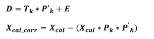
In the context of a transfer between instruments, the space of perturbations corresponds to the instrumental differences.
EPO – External Parameter Orthogonalization
External Parameter Orthogonalization (EPO) was the first orthogonalization method to be developed. Originally, it was created to remove perturbation parameters such as the temperature effect on spectral signals. It requires a balanced experimental design combining perturbation and concentration levels. It can be extended to inter-instrument transfer by considering the perturbation as inherent to the instrument. In this case, this EPO (External Parameter Orthogonalization) method is equivalent to the TOP (Transfer by Orthogonal Projections) method, which was developed in parallel specifically to address the calibration transfer problem, hence its more specific name.
In the case of multiple instruments, the spectra of each instrument are averaged. The average spectrum of one instrument is then subtracted from the others. The resulting matrix contains the variations related to the different instruments without any change in concentration. This matrix is decomposed using non-centered PCA (Principal Component Analysis) to extract k loadings, which are then used to orthogonalize the calibration matrix. The model must then be reconstructed, but it becomes instrument-independent and is therefore applicable to all instruments used for the transfer.
In the context of inter-instrument transfer, a standardization set is typically used to calculate the perturbation matrix D. The concentration does not need to be known because each sample is measured on the different instruments.
TOP – Transfer by Orthogonal Projections
The Transfer by Orthogonal Projections (TOP) method was developed more or less in parallel with the EPO (External Parameter Orthogonalization) method, but specifically for calibration transfer. The principle is to calculate the average of the spectra for each instrument from a standardization set; these averages are then concatenated. The resulting matrix D is then decomposed using centered PCA (Principal Component Analysis). A selection of k loadings is made to model the space related to instrumental differences. The calibration spectra are then orthogonalized with respect to this space. This method requires recalibration on the orthogonalized spectra. The resulting model is therefore instrument-independent.
EROS – Error Removal by Orthogonal Subtractions
The Error Removal by Orthogonal Subtractions (EROS) method is more recent. It was developed to reduce differences between replicas, but it is based on the same principle.
It has the advantage of generalizing the two previous methods, TOP (Transfer Orthogonalization Projection) and EPO (External Parameter Orthogonalization), by considering all spectral variations outside the concentration of interest. It is therefore more versatile because it can handle several types of perturbations simultaneously.
To do this, it is necessary to have either 1) a standardization set with the same sample measured under different conditions, thus using different instruments in our transfer application case; or 2) the concentration of interest value for each sample, in which case all samples with the same concentration are grouped together. Each set of samples at a given concentration is then centered on itself to remove the concentration-related information. All the sets are then concatenated into a matrix D, which therefore contains the instrumental variations (and possibly other variability factors). As with the other methods, a PCA (Principal Component Analysis) is performed on this matrix to calculate the spectral perturbation space, and then the calibration basis is orthogonalized to this space, thus becoming independent of the instrumental variabilities. The model reconstructed on this database is then applicable to the different instruments used for the transfer.
DOP – Dynamic Orthogonal Projection
The Dynamic Orthogonal Projection (DOP) method differs significantly from other orthogonalization methods. While the principle remains the same: orthogonalizing the calibration dataset with respect to the perturbation space. It was specifically developed to address the issue of updating online models, where obtaining reference measurements is quite complex. Thus, it aims to correct a drifting model using only a few calibration samples with their associated references, without requiring a standardization set.
In the context of data transfer between instruments, this “drift” can simply be the difference between the responses of the two instruments.
The method involves selecting spectra from the calibration dataset that have concentrations close to those of the calibration samples. Using a weighted (Gaussian) average calculation, virtual samples are reconstructed from the calibration spectra for each calibration sample. These are called virtual standards. Indeed, once these virtual standards are calculated, we find ourselves in the same situation as with a real standardization set, but with the spectra of the primary instrument reconstructed. The difference D between these samples is then calculated, and then, just as with the TOP (Transfer Orthogonalization Projection) method, PCA (Principal Component Analysis) is performed to decompose the inter-instrument differences into loadings representing the perturbation space. The calibration basis is then orthogonalized, and the model is reconstructed. As with the other methods, the model is then instrument-independent.
-
Process supervision methods
MSPC – Multivariate Statistical Process Control
SPC, Statistical Process Control, methods are widely used in order to supervise a process and detect any anomalies or drifts. However, SPC only looks at one parameter at a time, which makes monitoring complicated if the number of parameters to be followed is large; but this method is also less reliable because it does not take into account the interactions between the various variables of the process.
MSPC, Multivariate Statistical Process Control, makes it possible to control the processes in a multivariate way thus taking into account the globality of the process. It is usually based on PCA but other methods can also be used. Leverage and residue statistics are tracked to detect potential issues. Values beyond the statistical confidence intervals are considered as anomalies. It is then possible to return to the variable (s) causing the anomaly in order to diagnose the problem and be able to act quickly on the process.
MSPC can be performed on spectroscopic data (Near infrared, Raman ,…), analytical data (temperature, pressure, concentrations,…), or a combination of both.

BSPC – Batch Statistical Process Control
BSPC, Batch Statistical Process Control, is the equivalent of MSPC but for batch process control. The system is therefore more complex.
The most classic method is generally to compare the new batches to a “golden batch”, that represents a reference batch for which the conditions are controlled and optimal. This “golden batch” represents the nominal trajectory. The batches deviating from this trajectory can thus be detected, in the same way as for an MSPC model by following the scores, and / or the residuals and the leverage. It must therefore be well defined from several batches carried out under nominal conditions in order to achieve a robust model with relevant confidence intervals.
Although PCA is the most common method, multi-ways methods can also be used to follow the process, like for example the PARAFAC method, the data are indeed organized in 3 dimensions: batch x time x variables.
The BSPC faces various challenges including in particular the batch alignment so as to be able to compare them (different duration, key stages occurring at different points, etc.). Several methods make it possible to manage this problem according to the case : synchronization, temporal distortion, normalization, maturity index, etc. This step is critical when the objective is to compare with a “golden standard” and / or when multi-ways methods are used.

-
Design of Experiments
Design of Experiments
Using historical databases to model processes requires a very large amount of observations to ensure a minimum of variability. When it is possible, a more rational way consists in choosing the observations or experiments to span the whole desired operating conditions, i.e. the design space, with a maximum of variability. Design of Experiments (DoE) corresponds to that part of chemometrics which aims at planning the relevant experiments, minimizing the cost without decreasing information quality, quantifying the different factor effects, modelling and optimizing the processes.
Different designs correspond to different objectives:
- The DoE methodology often includes a first step which consists in implementing a screening design. The experiments are chosen in order to quantify the influential factors among a large number of factors.
- Full factorial designs are the basic designs which carry out all possible experiments with k two-level factors, low and high levels. All experiments at the boundaries of the design space are planned.
- Fractional factorial designs are used to screen factors when the number of experiments has to be lowered. The aliase principle allows selection of which experiments from the full factorial design must be running without loosing significant information.
Other screening designs using linear models are also commonly used to identify a few significant factors among many: The Plackett-Burman designs, The Rechtschaffner screening designs…

They talk about us
« Ondalys, a bridge between academic research and industry »
Our expertise to make sense of your data
With more than 15 years of experience in data analysis, Chemometrics and Machine Learning, especially applicated to spectroscopic data, our team helps you in each step of your project.
You need a tailor-made training ?
Our team study your request to offer you the most suitable and personalized training.